A Confused Look at Nicolas Cage Movies

May 10, 2020 6-minute read

The other day I watched Mandy (2018), a confusing Nicolas Cage movie that feels like an odd fever dream.
A few weeks ago, I watched Color Out of Space (2020), a confusing Nicolas Cage movie that feels like an odd fever dream, based on the Lovecraft story of the same name which I read a couple weeks prior.
So… yeah. That’s why Nic Cage has been on my mind a little lately.

Additionally, I’ve been trying to fiddle around with {ggplot2} themes a little more, because relying on {hrbrthemes} alone felt a little unsatisfying, and I thought it was time to make a theme that fits trakt.tv reasonably well.
And, while we’re at it, I saw these great {ggrepel} examples which is why I wanted to play around with {ggrepel} a little more.

And that’s where this post comes from, so here goes nothing.

I’ll start by loading all the things:

1
2
3
4
5
6
7
8


library(tRakt) # jemus42/tRakt
library(tadaathemes) # tadaadata/tadaathemes for theme_trakt()
library(ggplot2)
library(ggrepel) # >= 0.9.0
library(dplyr)
library(kableExtra)

plot_caption <- "Data from trakt.tv // @jemus42"

To take a look at Cage’s movies, I’ll first need to find him on trakt.tv – which is easy enough through the search. Once I have his identifiers (I’ll be using the slug because it’s nice and human-readable), I can use people_movies to get, well, the movies of this particular ~~people~~ person.

1

search_query("Nicolas Cage", type = "person")

1
2
3
4


## # A tibble: 1 x 7
##   type   score name         trakt slug         imdb      tmdb 
##   <chr>  <dbl> <chr>        <chr> <chr>        <chr>     <chr>
## 1 person  159. Nicolas Cage 15197 nicolas-cage nm0000115 2963

 1
 2
 3
 4
 5
 6
 7
 8
 9
10
11
12
13


if (file.exists("cage_credits.rds")) {
  cage_credits <- people_movies("nicolas-cage", extended = "full")
  
  saveRDS(cage_credits, "cage_credits.rds")
} else {
  cage_credits <- readRDS("cage_credits.rds")
}

cage_movies <- cage_credits$cast %>% 
  filter(
    runtime >= 80, votes >= 10,
    !stringr::str_detect(character, "(uncredited)|(voice)|(Himself)")
  )

The returned objects is a list of two tibbles, named cast and crew. I’m only interested in the cast bit, and I’ll filter out items where the character description indictaes Cage’s role was uncredited, it’s a voice role or he’s playing himself ¹. I’ll also exclude movies shorter than 80 minutes and those with less than 10 votes on trakt.tv, because I have to draw the line somewhere.

 1
 2
 3
 4
 5
 6
 7
 8
 9
10
11
12


cage_movies %>%
  arrange(desc(released)) %>%
  head(10) %>%
  select(year, title, character, runtime, rating, votes) %>%
  kable(
    caption = "The 10 latest Nic Cage movies",
    col.names = c("Year", "Movie", "Role", "Runtime (mins)", "Rating", "Votes"),
    digits = 1
  ) %>%
  kable_styling(
    position = "center"
  )

Table 1: The 10 latest Nic Cage movies
Year	Movie	Role	Runtime (mins)	Rating	Votes
2020	Kill Chain	Araña	92	6.4	380
2020	Color Out of Space	Nathan Gardner	111	6.4	1576
2019	Primal	Frank Walsh	97	6.5	692
2019	Grand Isle	Walter	97	6.3	238
2019	Running with the Devil	The Cook	100	6.7	1039
2019	A Score to Settle	Frank	103	6.5	987
2018	Between Worlds	Joe	90	5.8	448
2018	Mandy	Red Miller	122	6.3	2675
2018	211	Mike Chandler	86	6.1	1302
2018	Looking Glass	Ray	103	6.0	742

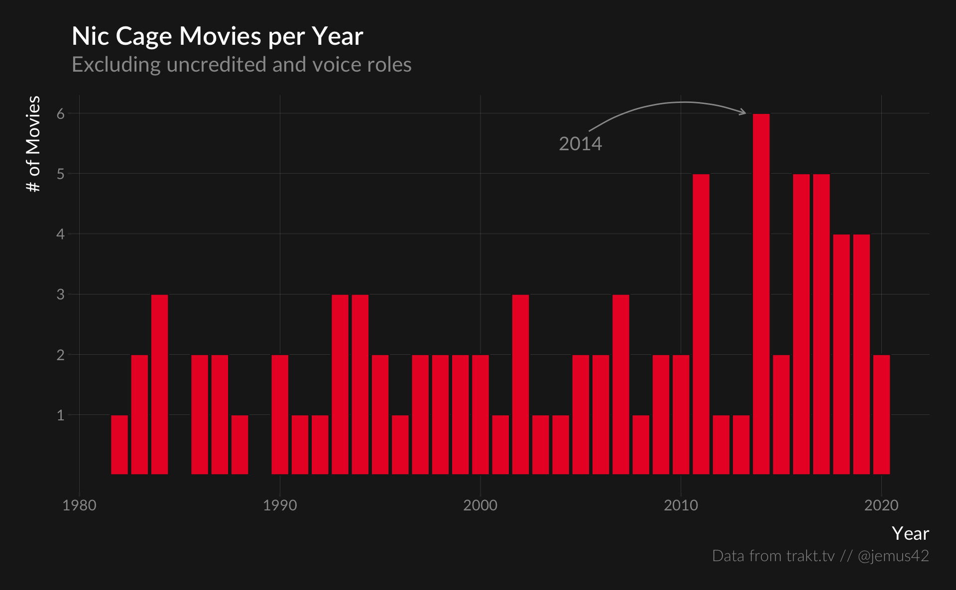
So, now I have some reasonably useful data. Let’s take a look at the number of movies per year:

 1
 2
 3
 4
 5
 6
 7
 8
 9
10
11
12
13
14
15
16
17
18
19
20
21


cage_movies %>%
  count(year) %>%
  ggplot(aes(x = year, y = n)) +
  geom_col(color = "#1D1D1D") +
  annotate(
    "text", x = 2005, y = 5.5, label = "2014", color = "#999999", size = 5,
    family = "Lato"
  ) +
  annotate(
    "curve", color = "#999999", curvature = -.25,
    x = 2005.4, y = 5.7, xend = 2013.2, yend = 6,
    arrow = arrow(ends = "last", length = unit(5, "pt"))
  ) +
  scale_y_continuous(breaks = seq(1, 10, 1)) +
  labs(
    title = "Nic Cage Movies per Year",
    subtitle = "Excluding uncredited and voice roles",
    x = "Year", y = "# of Movies",
    caption = plot_caption
  ) +
  theme_trakt()

Now the ratings for these movies, with a point size according to the number of votes cast:

 1
 2
 3
 4
 5
 6
 7
 8
 9
10
11
12
13
14
15
16
17
18
19
20
21
22
23
24
25
26
27
28
29
30
31
32
33
34
35
36
37
38
39
40


cage_movies %>%
  mutate(title_label = glue::glue("{title} ({year})")) %>%
  {
  ggplot(., aes(x = released, y = rating, size = votes)) +
  coord_cartesian(ylim = c(1, 10)) +
  geom_point(
    shape = 21, alpha = .75, fill = "#EA212D", color = "#1D1D1D"
  ) +
  geom_label_repel(
    data = filter(., rating < 4 | rating > 7.5),
    aes(label = title_label), 
    size = 4, color = "white", fill = NA,
    family = "Lato",
    force_pull = .5,
    box.padding = 4,
    point.padding = .7,
    label.padding = .5,
    label.size = 0,
    segment.color = "#999999",
    segment.curvature = -.25,
    segment.ncp = 2,
    segment.angle = 90,
    max.overlaps = Inf, max.iter = 10000,
    seed = 3236, show.legend = FALSE
  ) +
  scale_y_continuous(breaks = seq(1, 10, 1)) +
  scale_size_binned(guide = guide_bins(
    keywidth = unit(15, "mm"),
    axis.colour = "#999999",
    aesthetics = c("size", "point.size")
  )) +
  labs(
    title = "Nic Cage Movie Ratings on trakt.tv",
    subtitle = "By release date and number of votes",
    x = "Release Date", y = "Rating (1-10)",
    size = "Votes",
    caption = plot_caption
  ) +
  theme_trakt()
  }

And yes, I spent hours tweaking the {ggrepel} settings here, and at some point I gave up and called it good enough. I thought also mention that this plot highlights some of the weaknesses with the trakt.tv data – when it comes to ratings, especially for older items, it really shows that trakt.tv hasn’t been around for nearly as long as IMDb, and doesn’t even come close in terms of actively-rating-stuff user base. While I’m still sad about that, it doesn’t really matter that much for this little thing, but I thought I’d have to mention it.

Anyway, let’s take a look at the movies that have over 5000 votes, as a more or less arbitrary threshold for popularity:

 1
 2
 3
 4
 5
 6
 7
 8
 9
10
11
12
13
14
15
16
17
18
19
20
21
22
23
24
25
26
27
28
29
30
31
32
33
34


cage_movies %>%
  filter(votes > 5000) %>%
  mutate(
    title_label = glue::glue("{title} ({year})"),
    title_label = stringr::str_replace(title_label, ":", ":\n")
  ) %>%
  ggplot(aes(x = released, y = rating)) +
  coord_cartesian(ylim = c(1, 10)) +
  geom_point(
    shape = 21, alpha = .75, size = 5,
    fill = "#EA212D", color = "#1D1D1D"
  ) +
  geom_label_repel(
    aes(label = title_label), 
    size = 4, color = "white", fill = NA,
    family = "Lato",
    box.padding = 1,
    point.padding = .7,
    label.padding = .5,
    label.size = 0,
    segment.color = "#999999",
    segment.curvature = -.25,
    max.overlaps = Inf, max.iter = 10000,
    seed = 3236, show.legend = FALSE
  ) +
  scale_y_continuous(breaks = seq(1, 10, 1)) +
  labs(
    title = "Nic Cage Movie Ratings on trakt.tv",
    subtitle = "Excluding movies with a low number of votes",
    x = "Release Date", y = "Rating (1-10)",
    size = "Votes",
    caption = plot_caption
  ) +
  theme_trakt()

It’s a little too busy with the labels I think, but if you click on the plot to zoom it out, I think it at least does it’s job well enough.

Anyway, I think that’s about it for now, there’s a lot more that could be done with this little dataset, but I just wanted to play around with some stuff.

to which extent one might argue he’s always kind of playing himself is a different story ↩︎